In most microeconomics principles courses, the topics of costs and profit maximization come up towards the end of semester. This can be a challenge for students and faculty alike because of end-of semester workloads coupled with the rather abstract topics of short-run and long-run. This guide should help facilitate this learning process by increasing student’s attention and placing these concepts into a familiar light. We find out students are appreciative of any bridge between class concepts and the outside world. While the guide below is aimed at a principles course, it could also be useful in intermediate microeconomics theory courses.
Episode Title: Walt’s New Facility
Season: 3
Episode: 5
Episode Title: “Mas”
Timeframe: 21:13 — 25:30
Concepts: economics of scope, economies of scale, efficiency, elasticity of supply, fixed costs, fixed inputs, inputs, minimum efficient output, optimal output, production
Scene Summary
After Gus and Walter arrive an industrial-grade laundry facility, they enter a concealed passageway hidden under a dryer. The scene begins with the two entering the laboratory with an overview of the room and equipment (e.g., reaction vessels, mixing containers, and packages of various chemical ingredients) that follows. After the two proceed onto the laboratory floor, Walter exclaims “My God!” He then proceeds to investigate what lays underneath the bubble wrap akin to a child on Christmas Day. Thorium oxide for a catalyst bed and a 1,200-liter reaction vessel prompts Walter to ask how Gus was able to put everything together. Gus responds with:
“I had excellent help. […] Quite a lot of planning went into this. The laundry upstairs, I have owned it for years. It receives large chemical deliveries on a weekly basis, detergents and such. There is nothing suspicious about it and my employees, to be sure, are well-trained and trustworthy. The filtration system is state-of-the-art. It will vent nothing but clean, odorless steam, just as the laundry does and through the very same stacks”
Gus’s final response is the teachable moment. He notes that he needs “200 pounds per week to make this economically viable.”
Activity Summary
To illustrate the connection between short- and long-run average total costs and emphasize the planning curve concept, the following activity and discussion is best used after total and average total costs have been discussed, and the properties of average costs have been introduced. To illustrate the firm’s profit-maximizing behavior (i.e., finding the optimal output and price if discussing imperfect competition), the activity is best used after the topic has been explained at least once.
If this is to be used in an intermediate course, the activity can be used for recalling the concept of planning curve and the link between short- and long-run average total costs. This, in turn, facilitates the introduction of and a discussion about short- and long-run total costs, why the former is always larger than the latter, and, finally, the firm’s short- and long-run expansion paths.
Class Lecture
Prompt the class with the question of “From a firm’s perspective, what is the difference between the short and long run?” Students should point out that in the short run some costs are fixed while others are variable.
Follow up by asking “Why is it that there are fixed costs in the short but not in the long run?” This tends to take a little longer to elicit a response, but students should mention that in the short run some inputs are fixed (hence the fixed costs) while some are variable (hence the variable costs), but in the long run there are only variable costs. At this point, it is important to emphasize that once a firm invests in an input that is subsequently hard to adjust (i.e., plant size or capacity) it implicitly chooses a short-run total cost curve associated with that input.
After this initial conversation, show the scene Walt’s New Facility in its entirety. After the scene, ask students “Why did Gus not pick a laboratory of a smaller or larger capacity?” Students should be able to note that the size and the production capacity of the lab is determined by the size of the building that is concealing it, which in this case is an industrial laundry facility.
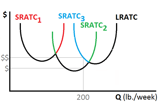
Next, the instructor should introduce Figure 1.1 below, which shows short-run average total cost curves (SRATC) associated with a small (red), medium (green) and large (blue) capacity laboratories:

After showing the graphs above, ask students why the short-run average total costs are higher with the small and large laboratories? At this point students should be able to quickly identify that an array of factors, ranging from the need of starting the production process multiple times (if the lab is small) to the risk of being discovered by the Drug Enforcement Agency (if the lab is large), dictate how small or large costs are.
Next, the instructor can reinforce a point made earlier, by choosing a certain production capacity/lab size, Gus has implicitly chosen to situate on the green short-run average total cost curve. The instructor can link the short- and long-run average total cost curves by introducing Figure 2 below:

At this point, it is also important to note that Gus could have chosen any production capacity/lab size but the constraints under which he operates pushed him towards the medium-sized lab. He may, nevertheless, revisit this decision and plan differently if the constraints change. However, this is possible only in the long run – after all, “Quite a lot of planning went into this.” Thus, the bottom of all possible short-run average total cost curves outline the long-run average total cost curve (i.e., planning curve).
One of the key points of the scene is that Gus mentioned needing 200 pounds per week to make his operation economically viable. Ask students to determine if they understand, given the previous charts, why Gus would make a comment like this. Students may need some time with this question but should eventually indicate that the costs associated with producing 200 pounds of methamphetamine per week are lower when using the medium-sized lab. Show students Figure 3 below to illustrate this cost difference:
Additional Lecture Material
This scene is also useful for discussing the firm’s profit-maximizing behavior. Ask students the same question mentioned in the previous section about why 200 pounds is the economically viable production level. Students should be able to point out that a weekly production of 200 pounds maximizes the profit if the point is at the intersection of marginal revenue and marginal cost curves. This can be shown as Figure 4 illustrates as long as the firm is a perfectly-competitive firm:
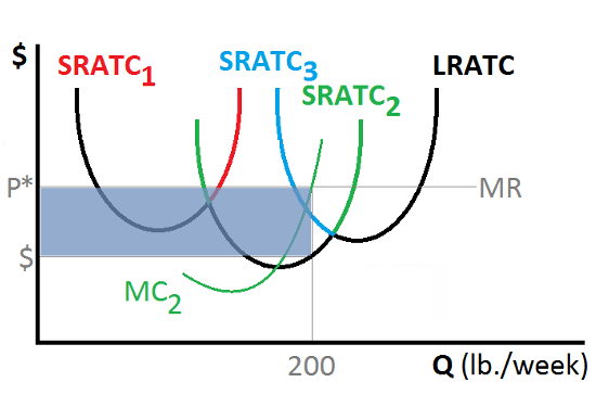
In the figure above, P* represents the market equilibrium price, MR denotes the marginal revenue, MC2 is the marginal cost curve associated with the medium-sized lab, and the shaded rectangle indicates the weekly profit generated by Gus’ drug business. For simplicity, the discussion above refers to perfectly competitive markets, but it can be adjusted to firms that operate in markets with imperfect competition.
Given the highly differentiated methamphetamine that Walter produces, the example is ideal for discussing how monopolistically competitive firms maximize profits. Figure 4 could also be used to motivate a discussion about profits as an incentive for market entry in the long run. The instructor can proceed by asking what students would expect to happen in this market if Gus’s enterprise is generating large enough profits.
In an intermediate microeconomic theory course, Figure 2 serves as a departure point in discussing why long-run average and total costs are equal or lower when compared with their short-run counterparts. A short explanation of this phenomena is tied with a more efficient production (and lower costs) when firms are able to choose the optimal bundle of inputs conditional on the desired level of output. A longer explanation should start with a discussion and the graphing of the firm’s short- and long-run expansion paths. Eventually, this should transpire into observing that, as the firm chooses among different level of outputs, picking the cost-minimizing bundle of inputs is possible only in the long run.
Extended Discussion Topics
- Constraints that firms face when purchasing fixed inputs
- Factors that shape these constraints. For example, current and future market demand, current and future availability of various technologies, access to financing, regulatory certainty, the importance of having and enforcing property rights.
- Short- and long-run time horizons differences across different industries
